First Prototype Revision

---

💡 Contribution of the hardware to address the necessity to develop a synthetic FRET biosensor of emerging contaminants.

A FRET (Förster Resonance Energy Transfer) biosensor can aid the detection of emerging contaminants by exploiting the principles of energy transfer between two fluorescent molecules; therefore, the main goal of hardware is to create an affordable device to monitor and classify the fluorescence the system emits (Medintz, I. L. et al., 2013)

Firstly, we need a way to excite the chromophore at a specific wavelength and measure the resulting fluorescence signal at a different specific wavelength. The first trials were carried out with fluorescent protein mCherry to help create a model to test the effectiveness of our fluorometer.

According to the mCherry spectrum (Figure 1), its peak absorption spectrum is between 580-590 nm. Both yellow (570-590 nm) and orange (585-620 nm) light have a wavelength that covers this desired peak (Opel et al., 2015), meaning that our excitation source must emit either of them. When talking about light sources, Light-Emitting Diodes (LED) are commonly employed, due to easy access and usage. As a first step in this project, orange light was selected as our emitting source due to the fact that its spectrum covers a larger part of the mCherry absorption spectrum.

🌟 Fluorescence detection with a Light dependent resistor

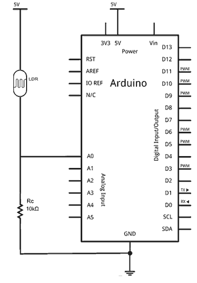
A sensor will allow us to probe the emitted fluorescence signal and any possible variation that may occur in the system. For this, a light dependent resistor (LDR) was chosen. An LDR will allow us to see how the fluorescence signal emitted by the fusion construct changes in the presence of the target cofactor. It is important to note that resistance on its own is not informational, but the voltage variations can be read using an analog input with a microcontroller. The LDR used for this was a GL5549, which is a 10 kΩ photoresistor. An LDR is a device that decreases its resistance when the light inciting over it increases, defining resistance as the opposition of current flow in an electrical circuit. This interaction can be described using Gustav Kirchhoff's reformulation of Ohm's law (1):

$$\mathrm{V\; =\; IR}$$

(1)

Where $\mathrm{V}$ is the voltage measured in a conductor, $\mathrm{I}$ refers to the current through the conductor and $\mathrm{R}$ the resistance of the conductor (Tenny, 2017). Another important concept is the ratio between illuminance and resistance which is explained as a potention function (2) (Nasrudin et al., 2011):

$$\frac{I}{I_0}={\left(\frac{R}{R_0}\right)}^{\mathrm{-ɣ}}$$

(2)

$I_0$ and $R_0$ represent known resistances and $\mathrm{-ɣ}$ is the slope of the log graph which shows the resistance losses by decade (Figure 2).

🔌 Electrical Schemas

A LED is a light-emitting diode that allows the passage of current in one direction, so it is considered a polarized device. Figure 4, shows that a LED is made up of an anode or the long leg, and a cathode or the shorter leg. The anode is where oxidation occurs, while reduction happens at the cathode, which indicates the direction of electron flow. In other words, the anode is where electric current enters a device, while the cathode is where it exits; these are denoted with positive and negative signs, respectively.

It is necessary to apply a specific voltage to the diode to achieve a forward polarization that allows current to flow freely with negligible resistance. However, when the polarization voltage is exceeded, a large current is produced that can damage the diode. To prevent this, a resistor was used to limit the amount of current passing through the LED (Bourget, C. M., 2008). The nominal current and polarization voltage of the LED values needed to calculate the resistor's value can be found online or on the LED's datasheet.

These parameters are the same as the voltage provided by our 5 V alimentation source. For an orange LED, the polarization voltage is 2.1 V, while the desired current is approximately 17 mA (Ozuturk, E., 2015). With these values we can estimate the value of the resistor as follows:

$$V=V_{\mathrm{cc}}-V_d=R\times I$$

(3)

$$5V-2.1V=R\times 0.017A$$

(4)

$$\frac{5V-2.1V}{0.017A}=170.6\Omega$$

(5)

There are two main considerations when choosing the resistor to use in a system:

• Use commercial resistor values.
• Use a bigger resistance than the one calculated to avoid damage to the LED in case of miscalculation or error.

While there aren't specific resistors for 170.6 Ω, we can use 180 Ω resistors, which is the closest commercial value. However, the current we would get from using these resistors is close to our desired current of 16 mA. As it is better to go for a larger resistor to avoid LED damage, the next available ones are 220 Ω, which may be more appropriate as the current it provides is closer to 14 mA.

The electrical schema for a LED and for the LDR are shown in Figures 4A and 4B respectively.

The use of a microcontroller is essential for providing a voltage source and reading the voltage across the sensor. Arduino will be the microcontroller for this device due to the ease of operation and the amount of libraries and documentation available. Arduino is an open-source electronics platform based on easy-to-use hardware and software (Arduino, 2018). The boards are able to read inputs and turn it into an output.

🔋 Reading Voltage

As shown in Figure 4, the use of a LDR in series with a 10 kΩ resistor was designed to create a voltage divider (6). Taking Figure 4 as a baseline, the LDR will be termed 'R1', the 10 kΩ resistor will be 'R2', the voltage output will be 'V_out':

$$V_{\mathrm{out}}=V_{\mathrm{in}}\left(\frac{R2}{R1+R2}\right)$$

(6)

$$V_{\mathrm{out}}=5V\left(\frac{10k\Omega }{R1+10\mathrm{k\Omega }}\right)$$

(7)

With these equations we are only left with the value of R1 which will change according to the value of the LDR. With no light input, R1 will be 10 kΩ, meaning the max V_out would be 2.5 V. On the other hand, as more light is sensed by the LDR, R1 decreases and the value of V_out will increase above 2.5 V. It is important to emphasize that these are theoretical values, a characterization component would be necessary to adjust the model and make correct predictions.

🚗 First Prototype Model

In Figure 6 we see the Eppendorf tube loaded with the sample and the LED illuminating through the Eppendorf. The LDR was placed 90º from the sample as it is where it can be closest to the protein without being directly affected by the LED. The excitation source must be in a place that allows us to direct the emission angle to avoid any noise on the LDR.

3D model development of this first prototype was carried out in SolidWorks (Figure 7A, 7B), and then printed using UltiMaker Cura and a 3D printer (Figure 8).

🔮 First Prototype Results

As orange light has a high wavelength, it belongs to a low energy spectrum. Meaning that the light emitted by mCherry as a response had less energy, definitely above its emission spectrum.Therefore, no significant differences between excited and unexcited signals were presented. Additionally, given that both its excitation and emission spectra remain within the visible light spectrum, any incident light would cause noise in the reading.

Taking the results from the first prototype, certain aspects needed to be reworked. First, the excitation source needed to be of a higher energy. Second, the device needs to be a closed system to avoid any light signals from the outside and increase accuracy. Lastly it is necessary to create a good generalization model that will work with any fluorescent signal and not just mCherry.

Second Prototype Revision

---

As this device is intended to be used with different types of fluorescent proteins and measure the intensity of its fluorescence signal by using a color sensor with white light emission, specifically the TCS230-Programmable Color Light-to-Frequency converter (TAOS™) shown in Figure 9A and B.

The TCS230 sensor includes a photodiode array, and a current-to-frequency converter that outputs a digital frequency as shown in figure 10. The sensor works with a supply voltage of 2.2 to 5.5 V (TAOS, 2011).

🔧 Photodiode Array

In the TCS230, the light-to-frequency converter reads an 8 x 8 array of photodiodes. Sixteen photodiodes have blue filters, 16 have green filters, 16 have red filters, and 16 are clear with no filters. The photodiode works based on the photoelectric effect, which states that when photons from a light source hit a semiconductor inside the diode, a current is generated. The photodiodes with filters will only detect photons with a frequency corresponding to the color wavelength (TAOS, 2011). The detection peak for each photodiode is shown in the responsivity graph in Figure 11.

The four colors of photodiodes are interdigitated to minimize the non-uniformity effect of incident irradiance. All photodiodes of the same color are connected in parallel. Pins S2 and S3 are used to select which group of photodiodes (red, green, blue, clear) are active.

📺 Current to Frequency Converter

Once the photodiodes convert incident light to current, the TCS230 module converts the current to frequency, which can be then transformed into a square wave, with a pulse generator that can be then read by a microcontroller. In Figure 12 the basic circuit for a current-to-frequency converter is shown. Pins S0 and S1 are used to select the range of frequencies (0 - 12 kHz, 0 - 120 kHz or 0 - 600 kHz) at which you want the converter to work.

The device can output up to 600 kHz before saturation. However, under normal conditions (supply voltage = 5 V, Temperature = 25 °C), when tested under 470 nm (blue), 524 nm (green), and 640 nm (red) wavelengths, the clear diodes reach only 13 kHz, while each colored diode reach 80 % of this value when exposed to its corresponding light (TAOS, 2011).

In general, the output is a square wave (50 % duty cycle) with frequency directly proportional to light intensity (TAOS, 2011). Since most objects do not emit their own light, the entire module is equipped with four white leds so their light bounces off the object and the sensor can detect the color of said object.

📟 Microcontroller

Red, green and blue photodiodes were used as these are the three primary colors from which every other color can be derived. This is known as the RGB model, which is used in almost every digital screen. Luminescence of each RGB component is directly proportional to frequency, where a lower frequency translates into a higher color intensity and vice versa. The frequency output can be read by the microcontroller which will transform the information into a serial output that can be read and manipulated in MATLAB to obtain the RGB components of a certain color. For this prototype the microcontroller Arduino Nano was used, Figure 13 has the electrical schema.

While the sensor can output up to 13 kHz under perfect conditions, tests were needed to determine the practical maximum and minimum frequency values under the prototype's normal conditions of operation. This was done by obtaining readings with white and black substances inside the Eppendorf tube, as white in the RGB color model is made by mixing red, blue, and green light at full intensity, while black is obtained by mixing their lowest intensity values (Ibraheem, 2012).

With the calibration values for maximum (Max_f) and minimum frequency (Min_f) set, a MATLAB script was created to map the frequency value read by the sensor and into a new value range from 0 to 255 using formula 8.

$${\mathrm{RGB}}_{\mathrm{value}}=\frac{\mathrm{Frequency}-{\mathrm{Min}}_f}{{\mathrm{Max}}_f-{\mathrm{Min}}_f}\cdot 255$$

(8)

This process was repeated for each RGB component and is explained in more depth in the Modeling and Device Calibration section. These three values were charted into an RGB color wheel to obtain the color detected by the sensor. The different fluorescence signals produced can be used to determine which protein is being detected. After obtaining the RGB values at different concentrations, they were plotted to observe the changes in RGB value when the concentration of a certain protein changes. This curve was then used to predict the concentration of any fluorescent protein.

🚗 Second Prototype Model

The second 3D printed model is shown in Figure 14. A dark chamber to avoid noise produced by external light and a compartment for the color sensor were added. This prototype was developed and printed following the same procedure as the first prototype.

🔮 Second Prototype Results

For the calibration, sunscreen was put as a test sample to obtain readings for white values. To obtain readings for black values, tests were run on the closed empty box. The frequencies obtained under these two conditions are registered in Table 1.

Table 1. Calibration values for second prototype

	R	G	B
White (Min)	33 Hz	57 Hz	63 Hz
Black (Max)	280 Hz	304 Hz	250 Hz

After calibration, the device was tested with mCherry diluted to different concentrations (1:3, 1:1, 3:1 and pure mCherry) obtaining its RGB values.

In the dispersion graph (Figure 15) a lineal change can be observed between the protein concentration and its RGB values, especially for the red value. The color measured was closer to purple than red, which is the color of mCherry when not excited. These results suggest that color can be used to determine the concentration, however, this white-light approach does not allow differentiation between fluorescence signals as only the color of the sample is being measured.

Third Prototype Revision

---

Following the failure of using orange light as an excitation source a higher energy source out of the light spectrum is needed to induce a fluorescent response. The mCherry excitation spectrum, (Figure 1) shows a higher energy excitation peak around 300-400 nm (UV light), which may be the key to produce a fluorescent response.

Before making significant changes to the model, it was necessary to prove that UV light can effectively produce a fluorescent response in the protein.

☀️ UV Light as an excitation source

In order to enhance the calibration of the device model, in addition to the mCherry protein, enhanced Green Fluorescent Protein (EGFP) will be included as part of the system calibration.

Figure 16 shows vials with different dilutions of mCherry and their fluorescence when exposed to a UV-transilluminator in a dark room.

As it can be seen, a fluorescence response is triggered by the UV light in mCherry. However, this does not mean that EGFP will react in a similar way.

EGFP's emission and excitation spectra shows that there is significant absorption around the UV-light range.

🚗 Third Prototype Model

The purpose of the device is try to emulate the behavior observed in the transilluminator (Figure 16B, 18B) for any sample, and then measure that response with the use of a color sensor RGB (TCS230-Programmable Color Light-To-Frequency Converter, TAOS™). Correct signal detection by the TCS230 depends on light that bounces off the sample after illuminating it with the white LEDs of the integrated circuit.

As UV-light became a necessity for the device, UV-light LEDs (Steren® 5 mm UV LED) were added to the model. To accommodate this, modifications were made to the CAD model (SolidWorks), where two gaps were incorporated so that LEDs could be inserted as shown in Figure 19.

After testing the device by introducing samples of pure mCherry and EGFP we could see the fluorescent response of both proteins (figure 20) which resembles the behavior of those previously tested in the transilluminator (Figure 16 and 18). This confirmed that UV-light was required to produce a detectable fluorescence signal and allowed us to quantify the difference between the color of an excited sample and one that is not.

🔮 Third Prototype Results

The interaction between sample-emitted light, the UV-light and the white LEDs of the sensor caused some noise as the white- and UV-light were clashing with each other. The sensor doesn't include an option to turn off the light incorporated in the circuit. Once a power source is connected the sensor LEDs turn on, so they were covered with tape.

It was observed that the range of the sensor was limited, since it was only able to make a measurement when the Eppendorf tube was directly in contact with it. This is a problem because as the sensor gets closer to the sample, the UV light also needs to be closer to the sample due the range of the LED, becoming a source of noise.

The TCS230 color sensor was discarded due to the inability to control the on-off state of its white LEDs, and the fact that it did not work when the sample was more than 1 mm away from the sensor when the white LEDs were covered with insulating tape.

Final Prototype Revision

---

🌈 Color Sensor TCS34725

After revising different market options, we decided to use the color sensor TCS34725 (Color Light-to-Digital Converter with IR Filter TCS34725, TAOS™) (Figure 21A, 21B). This sensor allows the user to turn the white led on and off, program its analog gain and integration time, block infrared (IR) light, and set manual interruption thresholds.

The TCS3472 light-to-digital converter contains a 3 x 4 photodiode array, four analog-to-digital converters (ADC) that integrate the photodiode current, data registers, a state machine, and an I2C interface. The 3 x 4 array is made up of red-filtered, green-filtered, blue-filtered, and unfiltered photodiodes. Additionally, the photodiodes are coated with an IR-blocking filter (TAOS, 2012) and have a particular responsivity under normal conditions (supply voltage = 5 V, Temperature = 25°C) (Figure 22).

The four integrating ADCs simultaneously convert the amplified photodiode currents to a 16-bit digital value. Upon completion of a conversion cycle, the results are transferred to the data registers, which are double-buffered to ensure the integrity of the data. All of the internal timing, as well as the low-power wait state, is controlled by the state machine (TAOS, 2012). Unlike the TCS230, the currents are not converted into frequency, instead they are directly converted to a digital value and sent to the microcontroller through a fast, up to 400 kHz, two-wire I2C serial bus. The TCS34725 provides a separate interrupt signal output. When interrupts are enabled, and user-defined thresholds are exceeded, the active-low interrupt is asserted and remains that way until it is cleared by the controller. This interrupt feature simplifies and improves the efficiency of the system software by eliminating the need to poll the TCS34725 (TAOS, 2012).

This sensor can be supplied with either 3.3 V (3V3 pin) or 5 V (VDD). The I2C Serial Clock Input Terminal (SCL) and the Serial Data Input/Output terminal (SDA) pins are used to control I2C communication (Figure 23), and can be manipulated using Arduino (Figure 24). The ground (GND) pin is used to control the white led (figure 21). If it is not connected, the LED will turn on, if it is connected it will turn off and if it is connected to INT, its behavior can be manipulated through interruptions (TAOS, 2012).

🚗 Final Prototype Model

The Eppendorf tube that holds the sample needs to be as close as possible to the color sensor, and the sensor should be as isolated as possible from the UV light. Therefore, the RGB sensor was put on the side of the biosensor rather than on the bottom and the slot for the Eppendorf was added so that it could block as much UV light as possible. Additionally, 8 total UV-light LEDs were added to maximize protein fluorescence (Figure 25).

🔮 Final Prototype Results

The final device model included a TCS34725 color sensor with a white LED that can be turned on and off as well as the 8 UV-LEDs. There are 4 different situations that needed to be tested such as using the LEDs and the sensor light, using the LEDs but not the sensor light, and other situations. Table 2 shows the system's noise, where the data returned by the sensor was captured to see the differences between possible noise the system would produce for each sample.

Table 2. Noise values for fourth prototype

White LED off/UV off
Component	Min	Max
R	2	4
G	3	5
B	2	4
White LED on/UV off
Component	Min	Max
R	20	541
G	16	633
B	10	448
White LED off/UV on
Component	Min	Max
R	109	587
G	67	290
B	362	1618
White LED on/UV on
Component	Min	Max
R	129	1248
G	81	1139
B	374	2082

Following the same steps as in the second prototype's calibration, sunscreen was used to simulate maximum possible values and the closed box was used to simulate minimum possible values. From now on, the model will be used with the sensor's white LED off and the UV-light on since, ideally, the inside of the box is dark enough so the sample has no light to absorb. If the sample is exposed to white light, the measurement will be affected, hence, if we keep only the UV-light, the sample will emit a fluorescent response according to it. In Figure 26 a trial run with an EGFP sample can be appreciated, the measurement obtained can be graphically represented in MATLAB, mixing the 3 normalized (scaled between 0 and 255) RGB components of the sample (Figure 27).

There are visual and quantifiable differences between the proteins when induced and not indicating that the system worked correctly for both mCherry and EGFP. The use of the equation 8 allows us to not perceive samples that do not produce fluorescence, due to the fact that the UV-light inside is considered a basal state in the model (a.k.a. As our minimum value). This is because the minimum value is being subtracted from all the values and the minimum value of the system is considered the measurement for the UV-light inside, only those samples capable of producing disturbances to the UV value readings will be different to 0, but those values that do not produce any interference will remain similar to basal state and therefore be closest to 0.

📷 Supervised Learning Validation: Utility and Functionality of the Hardware

RGB values have been used in image processing for some time and it's one of the most used color models, usually with its values mapped from 0 to 255 so they can be stored in a single byte of memory, forming a three-dimensional matrix where each array represents one of the three components of the model (Figure 28) (Dutta S., 2009).

The TCS34725 returns color component values, but it doesn't return values in the range of 0 to 255 as it is not mapped between a maximum and a minimum. When the device is fully closed, the measurement tends to be 0 as there is no incidence of light. When we turned on the UV-light, the values measured were close to 170, 68 and 492 (R-G-B respectively) on average, concluding that UV-light is mostly composed of red and blue on the visible spectrum, differences can be appreciated in Table 2.

Is needed to declare the minimum and maximum values the device will be able to measure in each component to normalize values between 0 and 255 as shown in Figure 27, understanding the lowest value of 0 corresponding to black and 255 to white. UV-light is being used to induce fluorescence in the sample, therefore, every evaluation will be biased by this incident light.

Table 3. Example Calibration Values.

Tests
Component	UV off	UV on	EGFP with UV off	EGFP with UV on
R	0	170	4	217
G	0	68	8	314
B	0	492	3	623

A significant difference between the values for EGFP with both controls is shown in Table 3. In a similar sense, the UV-light itself is sufficient for the sensor to make a reading. Meaning that the measurement for EGFP made with UV-light is biased by the presence of UV-light. As we can measure the interference produced, we can subtract the incidence of UV-light to the EGFP gauge, keeping only the light emission EGFP produces. For now, these estimations are of no use, as we have not established maximum or minimum values.

To calibrate the system a large dataset is needed with RGB information for different proteins. Afterwards, a K-Nearest Neighbors (KNN) Supervised Learning algorithm will be implemented to create a classification machine learning (ML) model. An ML model is required to predict future measurements and declare incoming results from different samples from one of the proteins used to train the model.

Enhanced Cyan Fluorescent Protein (ECFP), Yellow Fluorescent Protein (YFP), Green Fluorescent Protein (GFP), and Red Fluorescent Protein (RFP) will be used to calibrate the device. ECFP was cloned into pET28b(+) (kanamycin selection) following the same protocols used for ECFP-EryK-mVENUS and AtPCS. Then, ECFP_pET28b(+) was transformed in E. coli BL21 and induced using 0.4 mM IPTG. The inducible proteins RFP (chloramphenicol selection), GFP (carbenicillin selection) and YFP (carbenicillin selection) were donated by Tecnológico de Monterrey campus Estado de México.

All bacterial strains were grown during their induction proceeding. After induction, cells were harvested and resuspended in 1 mL of M63 (My Biosource) culture medium supplemented with 0.1 µM thiamine, 1 mM MgSO₄ and the selection antibiotic (kanamycin, carbenicillin or chloramphenicol). This procedure was repeated to wash the cells and two different samples for each protein were made, where the cellular density of samples were fixed to OD₆₀₀ 3 and 5 (Figure 29).

As M63 culture medium is present in all samples, it was defined as the basal state and therefore its results are our minimum value. The possibility of M63 producing an effect under UV-light has to be considered. Fifty different measurements of M63 under UV-light were recorded and averaged to reduce the effect of a possible error in a sample. Maximum value was obtained using a white LED. For each protein density sample, fifty different measurements were done, meaning we end up with a dataset of four hundred different observations (Figure 30), enough to create a KNN algorithm.

KNN is a non-parametric supervised learning classifier, meaning it doesn't make any assumptions about the underlying data distribution. It uses proximity to make predictions about the grouping of an individual data point, finding the 'K' nearest data points in the training dataset based on a distance metric, usually the Euclidean distance, Figure 31 serves as visual support for model interpretation. It should be noted that the number of neighbors (K) must be determined arbitrarily, where implementing cross-validation can help determine its value (Kramer, 2013).

👷🏻‍♂️ Implementing K-Nearest Neighbors

Due to the amount of documentation and libraries available to implement machine learning, Python was chosen for this task. As a first step, data has to be transformed and normalized using the minimum and maximum values following equation 8. The dataset is then split into a training set and a test set. By default, the training set is 75 % of the dataset meanwhile the remaining 25 % is used as a test set. This helps evaluate the accuracy and capability of generalization of the developed model. Then, a K-Nearest Neighbor object must be created in Python using the Scikit-Learn (Pedregosa et al., 2011) library and trained using the train set.

Nonetheless, the K parameter needs to be designated using cross-validation, a technique used to determine the parameters of the model, looking for the values that improve its performance.

In Figure 32A, the highest test set accuracy corresponds to a 3-Nearest Neighbors model, which ensures better performance and a model with better generalization capability. The model itself seems to have a good performance (up to 90% accuracy) no matter which 'K' value is used, but as the test set is composed of new data for the model, the 3-NN model is selected.

Figure 32B explains how the accuracy of the model can change due to the observations that form the training and test sets. Training and test sets are randomly made, but in Python it is possible to establish the same random state for every iteration, avoiding different results per run and guaranteeing the use of the same training and test sets, which will always return a 0.97 accuracy for a K of 3.

Table 4. Classification Report.

Protein	Precision	Recall	F1-score	Suppport
EGFP5	1	0.94	0.98	16
RFP5	0.83	0.83	0.83	6
YFP5	1	1	1	13
ECFP5	1	1	1	12
EGFP3	1	0.92	0.96	11
RFP3	0.94	1	0.97	16
YFP3	0.92	1	0.96	12
ECFP3	1	1	1	14

In addition to Figure 33, Table 4 includes particular statistics according to the results of the confusion matrix. Precision is referred to as a measure of how many positive predictions made by the model are correct (9), and recall, or sensitivity, as a measure of the actual positive instances the model has correctly predicted (10). On the other hand, F1-score shows the relationship between both, where an F1-score of 1 indicates an excellent precision and recall (11). Support refers to the number of observations that the test set had for each protein. Specificity can also be calculated, which turns out to be a relation between all of the instances that the model classified incorrectly as positive (12). From the results, precision, recall and F1-score are closer to one, meaning that the model tends to give good and accurate results for the eight different sample sets, where its weakness seems to be RFP5 but it can be explained by the number of observations for that particular sample.

$$\mathrm{Precision}=\frac{\mathrm{True\; Positives}}{\mathrm{True\; Positives}+\mathrm{False\; Positives}}$$

(9)

$$\mathrm{Recall}=\frac{\mathrm{True\; Positives}}{\mathrm{True\; Positives}+\mathrm{False\; Negatives}}$$

(10)

$$F_1=2\cdot \frac{\mathrm{Precision}\cdot \mathrm{Recall}}{\mathrm{Precision}+\mathrm{Recall}}$$

(11)

$$\mathrm{Specificity}=\frac{\mathrm{False\; Positives}}{\mathrm{True\; Negatives}+\mathrm{False\; Positives}}$$

(12)

Conclusions

---

It is necessary to accumulate a dataset with more data points corresponding to the RGB color components collected from the fluorescence signal of different proteins and a range of concentrations or optical densities to increase the generalization capability of the model. With our current results we can conclude that a K-Nearest Neighbors model is a good approach to predict data measured by the device, meaning that it can use other new information and samples of proteins, as long as these belong to the color spectra the model was trained with. But a larger dataset is needed in order to include new proteins or increase the generalization capability of the model. The final 3D model for the device can be appreciated in Figure 34, where different chambers were implemented to hide the electronics.

🚨 Perspectives to learn from user feedback

Future plans include using the device with the FRET-based biosensor developed by the laboratory team, and implementing the use of a smartphone interface to facilitate and enhance the use of the device. This interface will directly receive data from the microcontroller, ideally using a bluetooth connection. Unfortunately working with bluetooth has proven difficult and required some restructuring of the device, the electronics, and the power supply. So far the device is powered by the 5 V USB port of a computer, the implementation of a bluetooth device would remove the need to have a computer as a reading device, but alimentation issues must be solved as electronic arrangements need to be made to use a voltage eliminator.

Documentation of the hardware system to enable reproduction by other teams

---

Materials:

• PLA filament.
• 3D printer.
• Bakelite board (5x5 cm).
• 8 UV-light LEDs (390-400 nm).
• Arduino Nano board.
• 2 S-116 switches.
• 8 220 Ω resistors.
• Breadboard cable.
• Soldering iron.
• Solder paste.
• Lead and tin solder.
• TCS34725 Color Light-to-Digital Converter with IR Filter.

Steps:

1. Use Figure 36 as a guide for the next steps, together with Figure 24.


Figure 36. Circuit Design for LEDs connection.

2. Solder the Arduino Nano to the bakelite board, do not obstruct analog, voltage and ground pins.
3. Coming from the voltage pin, solder cable joining the pin and one of the horizontal rails in the bakelite board.
4. Repeat step four for the ground pin. Be sure to use the other horizontal rail.
5. Using electrical schematic in Figure 24 start cutting wire for the pins specified on it. Solder the cables (5 cm long is recommended) to the bakelite, let the other end free for now. For voltage and ground pins, solder one cable in each rail.
6. Use a resistor to create a connection between the voltage rail and a vertical rail, solder it and in the same rail solder a cable that will go to the anode of one of the LEDs. Repeat this step for the 8 LEDs. Be sure to let the cables long enough (5 cm is recommended).
7. Take the 8 free cathodes from the LEDs and solder them, this will make them share the same cathode. Be sure to let a cable come out of this connection, do not use it yet.
8. Solder the cable from step 7 to a vertical rail in the bakelite. Coming from that same rail, solder another cable to the middle leg of one S-116 switch.
9. From the same S-116 switch, wield a cable from the ground lane to one of its legs.
10. Going back to the connections made in step 5, follow the electrical schematic from Figure 24 and solder the cables to their corresponding legs in the TCS34725, except for the ground.
11. Use the ground cable left in step 8 and solder it to any vertical rail that is not being occupied yet. From that rail solder a cable connecting the rail and the middle leg of the other S-116 switch.
12. Wield a cable between one of the remaining legs of the S-116 switch to the ground lane.
13. In the last step electronics were finished. Figure 36 illustrates the connections made to this point.


Figure 37. Device's circuitry.

14. In order to develop a physical model, SolidWorks 2023, a 3D computer-aided design (CAD) software, was used. The model consists of seven pieces, individually designed, in order to identify them, they were labeled as follows:
1. Circuit Box (Figure 38A): Designed to store the integrated circuits for device instrumentation.
2. C-Cover (Figure 38B): Integration of the TCS34725 is possible with this piece, allowing it to be assembled individually.
3. Main Box (Figure 38C): This part has two main purposes: to assemble the eight UV LEDs, the slots were placed sideways, and to include a window that enables the user to observe a sample introduced into the device.
4. Top Cover (Figure 38D): An upper-cover designed to block any light source external to that contained in the device.
5. Back cover (Figure 38E): This piece completely covers the back of the TCS34725, providing isolation from the external light and protection to the external part of the module. In addition, two slots were added to incorporate a switch button to control the UV LEDs.
6. Eppendorf tube holder (Figure 38F): Designed to hold a 1.5-2mL Eppendorf tube inside the device.
7. Window lid (Figure 38): Covers the window when complete isolation of the system is desired.


Figure 38A. CAD pieces planes.


Figure 38B. CAD pieces planes.


Figure 38C. CAD pieces planes.


Figure 38D. CAD pieces planes.


Figure 38E. CAD pieces planes.


Figure 38F. CAD pieces planes.


Figure 38G. CAD pieces planes.

15. After each part is individually made, an assembly is created in the software to ensure that the parts satisfy the required dimensions and proportion.
16. The parts are printed individually on a 3D printer, with PLA filament.
17. Assembly of the device, implementation of the electronics.